Assignment 5 Answer Key
Question 1
Load the CPS data using:
cps <- read.csv("http://rtgodwin.com/data/cps1985.csv")
Part (a)
To estimate the model in R use:
summary(lm(log(wage) ~ education + gender + age + experience + gender*education, data=cps))
Coefficients:
                     Estimate Std. Error t value Pr(>|t|)
(Intercept)           0.53764    0.70887   0.758 0.448521
education             0.18311    0.11333   1.616 0.106753
gendermale            0.69499    0.20315   3.421 0.000672 ***
age                  -0.06472    0.11345  -0.570 0.568616
experience            0.07754    0.11355   0.683 0.494959
education:gendermale -0.03362    0.01531  -2.196 0.028545 *
---
Signif. codes:  0 ‘***’ 0.001 ‘**’ 0.01 ‘*’ 0.05 ‘.’ 0.1 ‘ ’ 1

Residual standard error: 0.4509 on 528 degrees of freedom
Multiple R-squared:  0.2769,	Adjusted R-squared:  0.2701
F-statistic: 40.44 on 5 and 528 DF,  p-value: < 2.2e-16
Part (b)
The estimated effect of education on wage is: 18.3% for women, and (0.18311 - 0.03362) 15.0% for men.
Part (c)
The interaction term is what allows for a diffenece in the effect of education on wages, between men and women. R has already tested the significance of this variable. With a p-value of 0.0286, the difference is statistically significant at the 5% level.
Question 2
Load the fish market data:
fish <- read.csv("https://rtgodwin.com/data/fish.csv")
The population model that we are trying to estimate is:
$\log (totqty) = \beta_0 + \beta_1 \log (avgprc) + \beta_2mon + \beta_3tues + \beta_4wed + \beta_5thurs + \epsilon$
Part (a)
Plot the data using something like:
plot(log(fish$avgprc), log(fish$totqty), xlab="log price", ylab="log quantity")
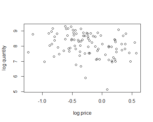
It doesn’t look like much of a demand curve. Each data point is actually the result of demand and supply intersecting, with both curves likely shifting around for each data point.
Part (b)
We can try to estimate the demand curve using LS, and add the estimated line to the plot:
ls.fish <- lm(log(totqty) ~ log(avgprc) + mon + tues + wed + thurs, data=fish)
abline(ls.fish)
(Don’t worry about the error message from abline()). The plot should look something like:

Part (c)
The IV model that we estimated in the book (using the ivreg() function) was:
install.packages("ivreg")
library(ivreg)
iv.fish <- ivreg(log(totqty) ~ log(avgprc) + mon + tues + wed + thurs |
                             wave2 + wave3 + mon + tues + wed + thurs,
                 data = fish)
summary(iv.fish)
Coefficients:
            Estimate Std. Error t value Pr(>|t|)
(Intercept)  8.16410    0.18171  44.930  < 2e-16 ***
log(avgprc) -0.81582    0.32744  -2.492  0.01453 *
mon         -0.30744    0.22921  -1.341  0.18317
tues        -0.68473    0.22599  -3.030  0.00318 **
wed         -0.52061    0.22357  -2.329  0.02209 *
thurs        0.09476    0.22521   0.421  0.67492
We need to reproduce these results using the two-stage least-squares (2SLS) approach. In the first stage, we regress the problematic endogenous variable on the instruments and all regressors (using least-squares), and then save the LS predicted values:
stage1.mod <- lm(log(avgprc) ~ wave2 + wave3 + mon + tues + wed + thurs,
                 data=fish)
logprice.fitted <- stage1.mod$fitted.values
In the second stage, we estimate the population model using least-squares, but we replace the variable $\log (avgprc)$ with the fitted values from the first stage:
stage2.mod <- lm(log(totqty) ~ logprice.fitted + mon + tues + wed + thurs,
                 data=fish)
summary(stage2.mod)
Coefficients:
                Estimate Std. Error t value Pr(>|t|)
(Intercept)      8.16410    0.18146  44.990  < 2e-16 ***
logprice.fitted -0.81582    0.32700  -2.495  0.01440 *
mon             -0.30744    0.22890  -1.343  0.18259
tues            -0.68473    0.22569  -3.034  0.00315 **
wed             -0.52061    0.22327  -2.332  0.02192 *
thurs            0.09476    0.22490   0.421  0.67451
---
The results are nearly identical to those obtained by the ivreg() function.