Assignment 2 Answer Key
Question 1
Download the data using:
mydata <- read.csv("https://rtgodwin.com/data/icecream.csv")
To estimate the model:
$revenue = \beta_0 + \beta_1temp + \epsilon$
and view a summary of the results, we can use:
summary(lm(revenue ~ temp, data=mydata))
##
## Call:
## lm(formula = revenue ~ temp, data = mydata)
##
## Residuals:
##     Min      1Q  Median      3Q     Max
## -26.000  -7.848  -1.526   7.106  26.231
##
## Coefficients:
##             Estimate Std. Error t value Pr(>|t|)
## (Intercept)  409.960      9.009   45.51   <2e-16 ***
## temp           3.848      0.356   10.81   <2e-16 ***
## ---
## Signif. codes:  0 '***' 0.001 '**' 0.01 '*' 0.05 '.' 0.1 ' ' 1
##
## Residual standard error: 11.09 on 140 degrees of freedom
## Multiple R-squared:  0.4549, Adjusted R-squared:  0.451
## F-statistic: 116.8 on 1 and 140 DF,  p-value: < 2.2e-16
The above output from the summary() function is ugly, and the person you are reporting your work to does not want to see it. You should make an effort to format the results, and pick out the important information, for example in a table:
| Estimate | Std. Error | |
|---|---|---|
| intercept | 410.0 | 9.009 |
| temp | 3.848 | 0.356 |
The estimated slope of 3.848 can be interpreted as follows: For every increase in temperature of $1^{\circ}C$, revenue increases by $3.85 on average.
Question 2
The $R^2$ for the model is 0.4549, meaning that 46% of the variation in revenue can be explained by temperature.
Question 3
A 95% confidence interval around $b_1$ can be calculated by the formula:
$b_1 \pm t_c \times s.e.(b_1)$
where $t_c$ is the 95% critical value from the t-distribution. To get this critical value use:
qt(0.975, 140)
## [1] 1.977054
We use 0.975 because we want the t-value that puts 2.5% area in the tail (5% area in both tails for the 95% confidence). We use 140 for the degrees of freedom ($n - 2$).
Now, the 95% confidence interval is:
3.848 - 1.977 * 0.356
## [1] 3.144188
3.848 + 1.977 * 0.356
## [1] 4.551812
So, the interval is $[3.14, 4.55]$. This interval contains all values for any null hypotheses involving $\beta_1$ that we will fail to reject at the 5% significance level.
Question 4
The hypothesis is formulated by:
$H_0: \beta_1 = 4$
$H_A: \beta_1 \neq 4$
The t-statistic for this hypothesis test is: $t = \frac{b_1 - \beta_{1,0}}{s.e.(b_1)} = \frac{3.848 - 4}{0.356}$
Calculate this in R:
tstat <- (3.848 - 4) / 0.356
tstat
## [1] -0.4269663
To get the p-value, we can use:
2 * pt(tstat, df = 140, lower.tail = TRUE)
## [1] 0.6700598
Note that we want the area in the left “tail” of the distribution, so in this case we had to use lower.tail = TRUE. We multiplied by 2 because $H_A$ is two sided.
With a p-value of 0.67 we fail to reject the null at the 10% significance level (or any common significance level).
Question 5
Perhaps people consume more ice cream on the weekends. We can estimate the effect of weekend on revenue using the model:
$revenue = \beta_0 + \beta_1weekend + \epsilon$
The R code to estimate the above population model is:
summary(lm(revenue ~ weekend, data = mydata))
##
## Call:
## lm(formula = revenue ~ weekend, data = mydata)
##
## Residuals:
##     Min      1Q  Median      3Q     Max
## -30.032  -7.112  -0.649   7.891  46.030
##
## Coefficients:
##             Estimate Std. Error t value Pr(>|t|)
## (Intercept)  501.315      1.217 411.791  < 2e-16 ***
## weekend       19.082      2.266   8.422 3.96e-14 ***
## ---
## Signif. codes:  0 '***' 0.001 '**' 0.01 '*' 0.05 '.' 0.1 ' ' 1
##
## Residual standard error: 12.23 on 140 degrees of freedom
## Multiple R-squared:  0.3363, Adjusted R-squared:  0.3315
## F-statistic: 70.93 on 1 and 140 DF,  p-value: 3.958e-14
$b_0 = 501.32$ and $b_1 = 19.08$. $b_0$ is the sample average revenue on weekdays. $b_1$ is the difference between the sample average revenue on weekends compared to weekdays. That is, the sample average revenue is 19.08 higher on weekends. The sample average revenue on weekends is $b_0 + b_1 = 501.32 + 19.08 = 520.40$.
Question 6
In other words, test the hypothesis that the revenue is the same on weekends as it is on weekdays. Although we estimated a difference of 19.08, this difference may not be significant given the variability of the estimator. The null hypothesis is $H_0: \beta_1 = 0$. This is the same as a test of significance of the dummy variable. R has already performed this test. The p-value is 3.96e-14, which is very small. We reject the null hypothesis at any significance level. Weekends appear to make a difference for ice cream sales revenues.
Question 7
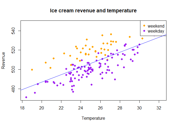
Since revenue is the dependent variable, it should go on the y-axis. We can put the continuous variable temp on the x-axis, and we can graph the dummy variable weekend by giving each data point a different colour based on whether $weekend = 1$ or $weekend = 0$.
First we create this variable to determine the colour of each data point:
mydata$mycol[mydata$weekend == 1] <- "orange"
mydata$mycol[mydata$weekend == 0] <- "purple"
Then we plot the data, add a legend, and add the estimated LS line to the plot:
plot(x = mydata$temp, y = mydata$revenue,
     main = "Ice cream revenue and temperature",
     xlab = "Temperature",
     ylab = "Revenue",
     pch = 16,
     col = mydata$mycol)

legend("topright",
       legend = c("weekend", "weekday"),
       col=c("orange", "purple"), pch=16)

abline(lm(revenue ~ temp, data = mydata), col = "blue")