Assignment 1 R code
This lab outlines the code that you need to do assignment 1.
Open RStudio
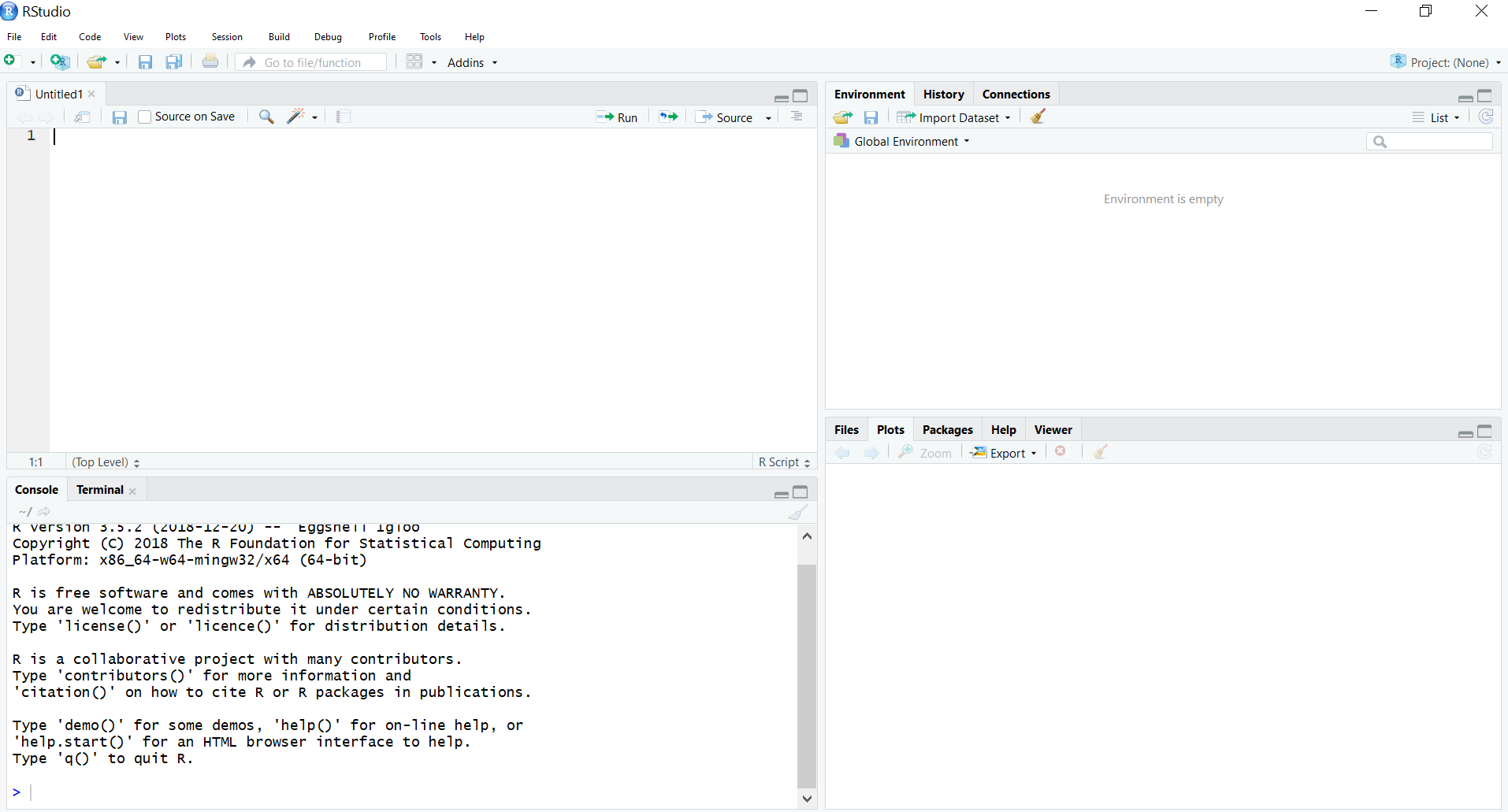
Search your computer for RStudio.exe and open the program. It should look something like this:
Create a script file
Click on “File”, “New File”, “R Script”.
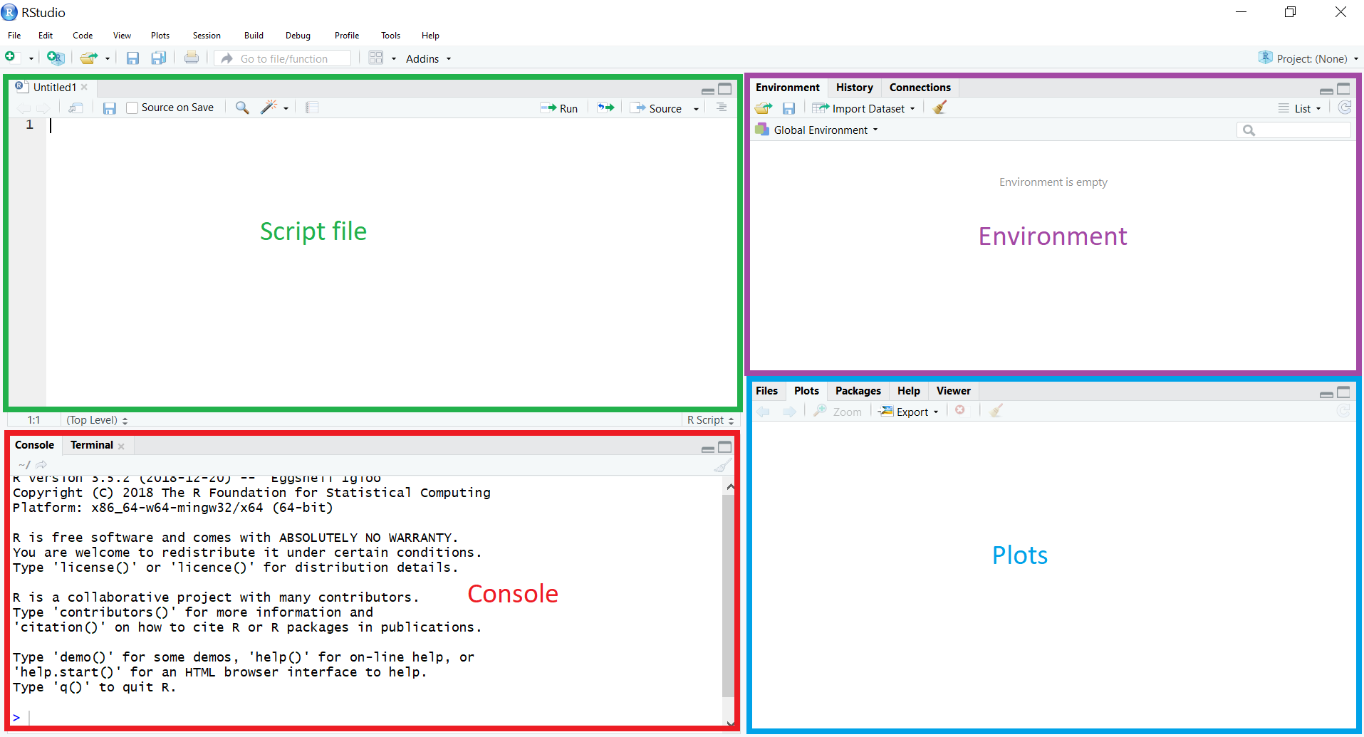
- In the top left is your Script file. R commands can be run from the R Script file, and saved at any time.
- In the bottom left is the Console window. Output is displayed here. R commands can be run from the Console, but not saved.
- In the top right is the Environment. Data and variables will be visible here.
- The bottom right will display graphics (e.g. histograms and scatterplots).
Load some data
There are several ways to load data into R. For this lab I will load the sample of heights from Chapter 3, directly from the internet (you can change the path in “quotations” to a file path on your own computer):
dat <- read.csv("https://rtgodwin.com/data/heights.csv")
Click on the “dat” object that shows up in the top-right “environment” window, and see that there is one variable in the data set called “heights”.
Calculate the sample mean (sample average)
    mean(dat$heights)

    ## [1] 174.085
Perform a t-test
To perform a t-test, we need to give the t.test() function the sample, and the null hypothesis. The function will estimate the standard error, determine the sample size, calculate the sample average. It will produce the t-test statistic, and a p-value:
t.test(dat$heights, mu = 173)


##         One Sample t-test
##
## data:  dat$heights
## t = 0.66627, df = 19, p-value = 0.5132
## alternative hypothesis: true mean is not equal to 173
## 95 percent confidence interval:
##  170.6766 177.4934
## sample estimates:
## mean of x
##   174.085
The p-value is 0.5132. This is greater than 10%, so we reject the null hypothesis at the 10% significance level.
(Note that in the text/lectures we calculated the p-value to be 44%. This is because we used the Normal approximation, which actually doesn’t work that well for a sample of 20).