Lab 4
Download the data
This lab uses life expectancy and health care expenditure data from Greene, example 6.10 (Greene, W. (2012). H.(2012): Econometric analysis. Journal of Boston: Pearson Education, 803-806). Download the data from the website using:
health <- read.csv("https://rtgodwin.com/data/health.csv")
Explore the data
The data is from 1997, and contains information on 191 countries with:
| Variable | Description |
|---|---|
| DALE | Disability adjusted life expectancy, in years |
| HEXP | Per capita health care expenditure |
| HC3 | Average years of education |
| OECD | A dummy variable =1 if country is in OECD, 0 otherwise |
| GINI | The GINI coefficient of income inequality |
| GEFF | An index measuring government effectiveness |
| VOICE | An index measuring the level of democracy |
| TROPICS | A dummy variable =1 if country is in the tropics, 0 otherwise |
| POPDEN | A measure of population density |
| PUBTHE | Proportion of health expenditure paid by bublic authorities |
| GDPC | GDP per capita |
In this lab, we want to investigate whether OECD countries are more efficient in their delivery of health care (DALE), through spending and education. That is, we want to see if the effect of HEXP and HC3 on DALE is different for OECD vs. non-OECD countries.
Before we can do this, we need to specify the right functional form. We need to see if there are non-linearities between the variables of interest.
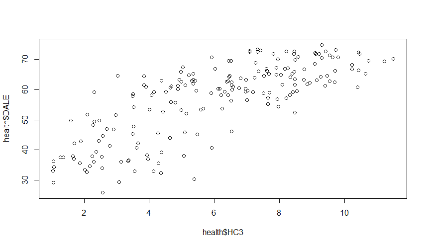
Create a plot of life expectancy and education:
plot(health$HC3, health$DALE)

There appears to be a possible non-linear (concave) relationship between education and life expectancy. To capture this, I will use a polynomial of HC3. Next, let’s look at a plot of life expectancy and health spending:
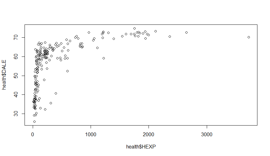
plot(health$HEXP, health$DALE)

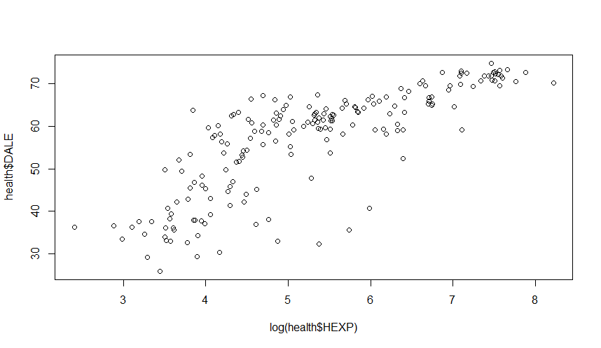
There is definitely a non-linear relationship here. It is possible that, instead of a dollar amount change in spending, a proportional (percentage) change in spending has a constant effect of life expectancy. To capture this idea, we take the log of spending:
plot(log(health$HEXP), health$DALE)

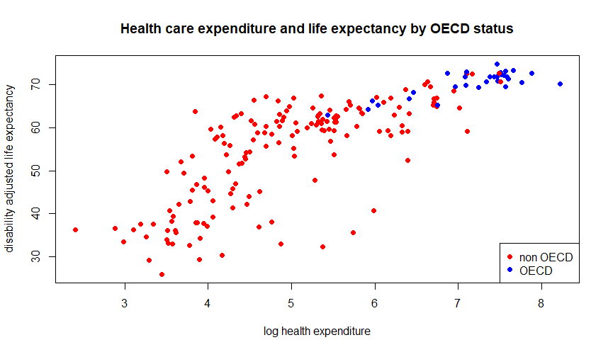
We have “linearized” the relationship! Before we start modelling, let’s colour-code the data point by OECD status:
health$col <- "red"
health$col[health$OECD == 1] <- "blue"
plot(log(health$HEXP), health$DALE,
     main = "Health care expenditure and life expectancy by OECD status",
     xlab = "log health expenditure", ylab = "disability adjusted life expectancy",
     pch = 16, cex = 1, col = health$col)
legend("bottomright", c("non OECD", "OECD"), pch = 16, col = c("red", "blue"))

From the plot, it is difficult to tell whether the effect of spending on life expectancy differs between OECD and non-OECD countries.
Estimate a model with interaction terms
In order to allow the effect of education and spending to differ by OECD status, we need to allow the OECD dummy to interact with the education and spending. We also need to allow for the non-linear relationship between the variables. To accomplish all this, we’ll estimate the model:
\[DALE = \beta_0 + \beta_1 \log(HEXP) + \beta_2 HC3 + \beta_3HC3^2 + \beta_4HC3^3\] \[+ \beta_5OECD + \beta_{13}[OECD \times log(HEXP)] + \beta_{14}[OECD \times HC3] + \beta_{15}[OECD \times HC3^2] + \beta_{16}[OECD \times HC3^3]\] \[+ \beta_6GINI + \beta_7TROPICS + \beta_8POPDEN + \beta_9PUBTHE + \beta_{10}GDPC + \beta_{11}VOICE + \beta_{12}GEFF + \epsilon\]In the model above, the 1st line contains the main variables of interest (health expenditure and education), the 2nd line contains the OECD dummy interacting with the main variables of interest, and the 3rd line contains the “controls” (variables that we may need to avoid omitted variable bias).
To estimate this model in R, we can use:
mod1 <- lm(DALE ~ log(HEXP) + HC3 + I(HC3^2) + I(HC3^3) + OECD + OECD*log(HEXP)
           + OECD*HC3 + OECD*I(HC3^2) + OECD*I(HC3^3) + GINI + TROPICS + POPDEN
           + PUBTHE + GDPC + VOICE + GEFF, data = health)
summary(mod1)
Coefficients:
                 Estimate Std. Error t value Pr(>|t|)
(Intercept)     2.596e+01  6.262e+00   4.145 5.30e-05 ***
log(HEXP)       5.364e+00  1.098e+00   4.885 2.33e-06 ***
HC3             3.779e+00  3.015e+00   1.253  0.21177
I(HC3^2)       -1.373e-01  5.940e-01  -0.231  0.81748
I(HC3^3)       -6.023e-03  3.545e-02  -0.170  0.86531
OECD            1.616e+01  8.266e+01   0.195  0.84525
GINI           -2.475e+01  7.091e+00  -3.491  0.00061 ***
TROPICS        -2.336e+00  1.164e+00  -2.007  0.04625 *
POPDEN          1.082e-04  1.813e-04   0.597  0.55148
PUBTHE         -2.528e-03  2.597e-02  -0.097  0.92258
GDPC           -1.834e-04  1.921e-04  -0.955  0.34097
VOICE           5.840e-01  8.521e-01   0.685  0.49406
GEFF            9.972e-02  1.091e+00   0.091  0.92731
log(HEXP):OECD -7.010e-01  2.527e+00  -0.277  0.78177
HC3:OECD       -1.119e+00  3.541e+01  -0.032  0.97484
I(HC3^2):OECD  -1.506e-01  4.516e+00  -0.033  0.97344
I(HC3^3):OECD   1.238e-02  1.870e-01   0.066  0.94730
---
Signif. codes:  0 ‘***’ 0.001 ‘**’ 0.01 ‘*’ 0.05 ‘.’ 0.1 ‘ ’ 1

Residual standard error: 6.17 on 174 degrees of freedom
Multiple R-squared:  0.7694,	Adjusted R-squared:  0.7481
F-statistic: 36.28 on 16 and 174 DF,  p-value: < 2.2e-16
Model selection
Order of the polynomial
The polynomial in HC3 is order 3 (it goes up to a cubed term), but it looks like the cubed term may be insignificant. To test to see if the cubed term is needed (if it’s insignificant), we actually need to perform a joint hypothesis test to see if both $HC3^3$ and $OECD \times HC^3$ are jointly insignificant. To do this, we can use the F-test. Estimate a model without the cubed terms (the restricted model), and compare the two models using the anova() function:
mod2 <- lm(DALE ~ log(HEXP) + HC3 + I(HC3^2) + OECD + OECD*log(HEXP)
           + OECD*HC3 + OECD*I(HC3^2) + GINI + TROPICS + POPDEN
           + PUBTHE + GDPC + VOICE + GEFF, data = health)
anova(mod1, mod2)
Model 1: DALE ~ log(HEXP) + HC3 + I(HC3^2) + I(HC3^3) + OECD + OECD *
    log(HEXP) + OECD * HC3 + OECD * I(HC3^2) + OECD * I(HC3^3) +
    GINI + TROPICS + POPDEN + PUBTHE + GDPC + VOICE + GEFF
Model 2: DALE ~ log(HEXP) + HC3 + I(HC3^2) + OECD + OECD * log(HEXP) +
    OECD * HC3 + OECD * I(HC3^2) + GINI + TROPICS + POPDEN +
    PUBTHE + GDPC + VOICE + GEFF
  Res.Df    RSS Df Sum of Sq      F Pr(>F)
1    174 6624.4
2    176 6625.6 -2   -1.1719 0.0154 0.9847
The p-value is very large (0.9847), so we fail to reject the null (the restricted model) that the cubed terms have no effect. Our new model is quadratic in education (goes up to the squared term):
summary(mod2)
Coefficients:
                 Estimate Std. Error t value Pr(>|t|)
(Intercept)     2.531e+01  5.025e+00   5.037 1.16e-06 ***
log(HEXP)       5.372e+00  1.079e+00   4.979 1.52e-06 ***
HC3             4.253e+00  1.100e+00   3.865 0.000156 ***
I(HC3^2)       -2.367e-01  9.325e-02  -2.539 0.011999 *
OECD            1.964e+01  2.497e+01   0.786 0.432680
GINI           -2.482e+01  7.029e+00  -3.531 0.000528 ***
TROPICS        -2.336e+00  1.157e+00  -2.020 0.044924 *
POPDEN          1.090e-04  1.800e-04   0.605 0.545702
PUBTHE         -1.865e-03  2.513e-02  -0.074 0.940942
GDPC           -1.835e-04  1.873e-04  -0.980 0.328595
VOICE           5.744e-01  8.454e-01   0.679 0.497767
GEFF            1.169e-01  1.079e+00   0.108 0.913862
log(HEXP):OECD -6.868e-01  2.278e+00  -0.301 0.763393
HC3:OECD       -2.808e+00  5.986e+00  -0.469 0.639549
I(HC3^2):OECD   1.040e-01  3.580e-01   0.290 0.771842
---
Signif. codes:  0 ‘***’ 0.001 ‘**’ 0.01 ‘*’ 0.05 ‘.’ 0.1 ‘ ’ 1

Residual standard error: 6.136 on 176 degrees of freedom
Multiple R-squared:  0.7693,	Adjusted R-squared:  0.751
F-statistic: 41.92 on 14 and 176 DF,  p-value: < 2.2e-16
Next, wee see if the squared terms are needed. We drop them from the model, and again perform an F-test where we compare model 2 and model 3:
mod3 <- lm(DALE ~ log(HEXP) + HC3 + OECD + OECD*log(HEXP)
           + OECD*HC3 + GINI + TROPICS + POPDEN
           + PUBTHE + GDPC + VOICE + GEFF, data = health)
anova(mod2, mod3)
Model 1: DALE ~ log(HEXP) + HC3 + I(HC3^2) + OECD + OECD * log(HEXP) +
    OECD * HC3 + OECD * I(HC3^2) + GINI + TROPICS + POPDEN +
    PUBTHE + GDPC + VOICE + GEFF
Model 2: DALE ~ log(HEXP) + HC3 + OECD + OECD * log(HEXP) + OECD * HC3 +
    GINI + TROPICS + POPDEN + PUBTHE + GDPC + VOICE + GEFF
  Res.Df    RSS Df Sum of Sq      F  Pr(>F)
1    176 6625.6
2    178 6876.0 -2   -250.46 3.3265 0.03819 *
---
Signif. codes:  0 ‘***’ 0.001 ‘**’ 0.01 ‘*’ 0.05 ‘.’ 0.1 ‘ ’ 1
With a p-value of 0.03819 we reject the null hypothesis (that the squared terms are not needed), and decide to keep the model with the squared terms (model 2).
Dropping insignificant variables
Several of the controls look insignificant. We test the null hypothesis that they are not needed by dropping them all (restricted model under the null), and then comparing them to model 2 (unrestricted model under the alternative hypothesis).
mod4 <- lm(DALE ~ log(HEXP) + HC3 + I(HC3^2) + OECD + OECD*log(HEXP)
           + OECD*HC3 + OECD*I(HC3^2) + GINI + TROPICS, data = health)
anova(mod2, mod4)
Model 1: DALE ~ log(HEXP) + HC3 + I(HC3^2) + OECD + OECD * log(HEXP) +
    OECD * HC3 + OECD * I(HC3^2) + GINI + TROPICS + POPDEN +
    PUBTHE + GDPC + VOICE + GEFF
Model 2: DALE ~ log(HEXP) + HC3 + I(HC3^2) + OECD + OECD * log(HEXP) +
    OECD * HC3 + OECD * I(HC3^2) + GINI + TROPICS
  Res.Df    RSS Df Sum of Sq      F Pr(>F)
1    176 6625.6
2    181 6709.3 -5   -83.706 0.4447 0.8167
With a p-value of 0.8167 we favour the restricted model (we fail to reject the null). The controls that we dropped are jointly insignificant. We now have the model:
summary(mod4)
Coefficients:
                Estimate Std. Error t value Pr(>|t|)
(Intercept)     25.34268    3.62726   6.987 5.20e-11 ***
log(HEXP)        4.81602    0.60615   7.945 2.00e-13 ***
HC3              4.42646    1.04809   4.223 3.81e-05 ***
I(HC3^2)        -0.24207    0.08979  -2.696 0.007684 **
OECD            22.82463   23.61794   0.966 0.335128
GINI           -22.58137    6.74951  -3.346 0.000998 ***
TROPICS         -2.20459    1.10996  -1.986 0.048522 *
log(HEXP):OECD  -1.60578    2.01375  -0.797 0.426259
HC3:OECD        -2.14219    5.86605  -0.365 0.715400
I(HC3^2):OECD    0.06755    0.35046   0.193 0.847381
---
Signif. codes:  0 ‘***’ 0.001 ‘**’ 0.01 ‘*’ 0.05 ‘.’ 0.1 ‘ ’ 1

Residual standard error: 6.088 on 181 degrees of freedom
Multiple R-squared:  0.7664,	Adjusted R-squared:  0.7548
F-statistic: 65.98 on 9 and 181 DF,  p-value: < 2.2e-16
Test the hypothesis that OECD countries are more efficient at producing life expectancy
We want to test if the effect of health care expenditure, and education, is different between OECD and non-OECD countries. To test this hypothesis, we can estimate two models. The unrestricted model mod4 has already been estimated above. The restricted model is obtained by dropping all of the interaction terms. The restricted model does not have interaction variables that allow OECD to have differeing effects:
mod5 <- lm(DALE ~ log(HEXP) + HC3 + I(HC3^2) + OECD + GINI + TROPICS,
           data = health)
anova(mod4, mod5)
Model 1: DALE ~ log(HEXP) + HC3 + I(HC3^2) + OECD + OECD * log(HEXP) +
    OECD * HC3 + OECD * I(HC3^2) + GINI + TROPICS
Model 2: DALE ~ log(HEXP) + HC3 + I(HC3^2) + OECD + GINI + TROPICS
  Res.Df    RSS Df Sum of Sq      F Pr(>F)
1    181 6709.3
2    184 6814.3 -3   -105.02 0.9444 0.4204
With a p-value of 0.4204, we fail to reject the null hypothesis (we choose mod5 in favour of mod4. We cpnclude that OECD countries are not more efficient than non-OECD countries, in terms of increasing life expectancy through education and health care spending.
Interpreting the coefficients
As an aside, let’s interpret some of the estimated coefficients from mod5.
summary(mod5)
Coefficients:
             Estimate Std. Error t value Pr(>|t|)
(Intercept)  24.85363    3.56998   6.962 5.74e-11 ***
log(HEXP)     4.60608    0.57572   8.001 1.35e-13 ***
HC3           5.07654    0.90346   5.619 7.01e-08 ***
I(HC3^2)     -0.30281    0.07346  -4.122 5.67e-05 ***
OECD         -1.27083    1.79905  -0.706  0.48084
GINI        -22.09751    6.65420  -3.321  0.00108 **
TROPICS      -2.31260    1.10483  -2.093  0.03770 *
---
Signif. codes:  0 ‘***’ 0.001 ‘**’ 0.01 ‘*’ 0.05 ‘.’ 0.1 ‘ ’ 1

Residual standard error: 6.086 on 184 degrees of freedom
Multiple R-squared:  0.7627,	Adjusted R-squared:  0.755
F-statistic: 98.59 on 6 and 184 DF,  p-value: < 2.2e-16
The estimated coefficient 4.60608 is interpreted as: a 1\% increase in per capita health care spending is associated with an increase in life expectancy of 0.046 years (about 17 days). Education has a positive (the sign on HC3 is positive) but diminishing (the sign on HC3sq is negative) effect on life expectancy. For countries with low levels of education the effect is large:
life.for.3.edu <- predict(mod5, data.frame(HEXP=100, HC3=3, OECD=0, GINI=.5, TROPICS=0))
life.for.2.edu <- predict(mod5, data.frame(HEXP=100, HC3=2, OECD=0, GINI=.5, TROPICS=0))
life.for.3.edu - life.for.2.edu
3.562519
For countries with only 2 years of average education, an extra year of education increases life expectancy by 3.5 years on average. In the above R code, we used mod5 to get LS predicted values for two representative countries (one with 3 years and one with 2 years), and took the difference. The other values that we chose for the “x” variables could be anything; the effects cancel out when we take differences.
We repeat the same procedure for a country with 8 years and 7 years of average education:
life.for.8.edu <- predict(mod5, data.frame(HEXP=100, HC3=8, OECD=0, GINI=.5, TROPICS=0))
life.for.7.edu <- predict(mod5, data.frame(HEXP=100, HC3=7, OECD=0, GINI=.5, TROPICS=0))
life.for.8.edu - life.for.7.edu
0.5344686
The effect has diminished to 0.5 years.