Lab 2
Background Story: A Monopolist’s Demand Curve
On Mars, Jim is the only person selling Earth rocks. There is no substitute for authentic Earth rocks, so Jim is a monopolist. Jim controls the price. Jim has tried changing the price of Earth rocks 132 times; for each price change, Jim recorded the quantity (in cubic cm) of Earth rocks sold for that day. Load the data into RStudio:
rocks <- read.csv("https://rtgodwin.com/data/monopolist.csv")
Explore the data
Look at the data in a spreadsheet (close the spreadsheet when done):
View(rocks)
There are three variables in the data. quantity is the amount of moon rocks sold on a day, price is the price set by the monopolist for that day, and bad.weather is a dummy variable equal to 1 if the weather on Mars was bad for that day, or equal to 0 if the weather was good.
Create a new variable to control the colour of each data point, based on the bad.weather dummy variable:
rocks$mycol[rocks$bad.weather == 1] <- "orange"
rocks$mycol[rocks$bad.weather == 0] <- "purple"
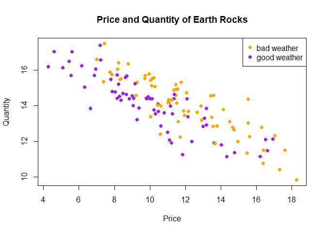
Plot the data. Put price on the x-axis, and quantity on the y-axis (so that the data depict an “inverse” demand curve), and use mycol to determine colour:
plot(x = rocks$price, y = rocks$quantity,
     main = "Price and Quantity of Earth Rocks",
     xlab = "Price",
     ylab = "Quantity",
     pch = 16,
     col = rocks$mycol)

legend("topright",
       legend = c("bad weather", "good weather"),
       col=c("orange", "purple"), pch=16)

Estimate the effect of an increase in price on quantity
To estimate the model $quantity = \beta_0 + \beta_1price + \epsilon$, we can use the lm() function:
lm(quantity ~ price, data = rocks)
Call:
lm(formula = quantity ~ price, data = rocks)

Coefficients:
(Intercept)        price
    18.7532      -0.4266
To get more information about the estimated model, such as the estimated standard errors and $R^2$, we need to put the lm() function inside the summary() function:
summary(lm(quantity ~ price, data = rocks))
Call:
lm(formula = quantity ~ price, data = rocks)

Residuals:
     Min       1Q   Median       3Q      Max
-2.45023 -0.60202  0.01372  0.68612  2.22578

Coefficients:
            Estimate Std. Error t value Pr(>|t|)
(Intercept) 18.75320    0.29292   64.02   <2e-16 ***
price       -0.42657    0.02576  -16.56   <2e-16 ***
---
Signif. codes:  0 ‘***’ 0.001 ‘**’ 0.01 ‘*’ 0.05 ‘.’ 0.1 ‘ ’ 1

Residual standard error: 0.9019 on 130 degrees of freedom
Multiple R-squared:  0.6784,	Adjusted R-squared:  0.676
F-statistic: 274.3 on 1 and 130 DF,  p-value: < 2.2e-16
Interpretation of the results
The estimated intercept is $b_0 = 18.75$ and the estimated slope is $b_1 = -0.43$. The estimated standard errors for $b_0$ and $b_1$ are 0.293 and 0.026, respectively. The interpretation of $b_1$ is: when price increases by 1, quantity demanded decreases by 0.43 on average.
$R^2 = 0.68$, meaning that price explains 68% of the variation in quantity.
Calculate a 95% confidence interval around the estimated slope
A 95% confidence interval around $b_1$ can be calculated by the formula:
$b_1 \pm t_c \times s.e.(b_1)$
where $t_c$ is the 95% critical value from the t-distribution. To get this critical value use:
qt(0.975, 130)
[1] 1.97838
We use 0.975 because we want the t-value that puts 2.5% area in the tail (5% area in both tails for the 95% confidence). We use 130 for the degrees of freedom ($n - 2$).
Now, the 95% confidence interval is:
-0.43 - 1.98 * 0.026
-0.43 + 1.98 * 0.026
[1] -0.48148
[1] -0.37852
So, the interval is $[-0.48, -0.38]$. This interval contains all values for any null hypotheses involving $\beta_1$ that we will fail to reject at the 5% significance level.
Hypothesis tests
Test the hypothesis that the demand curve is “flat” (i.e. price has no effect on quantity demanded).
Mathematically, this hypothesis is:
$H_0: \beta_1 = 0$
$H_A: \beta_1 \neq 0$
The t-statistic for this hypothesis test is: $t = \frac{b_1 - \beta_{1,0}}{s.e.(b_1)} = \frac{-0.43 - 0}{0.026}$
Calculate this in R:
tstat <- -0.43 / 0.026
tstat
[1] -16.53846
Since this t-stat is less than -1.97838, we know we will reject the null at the 5% significance level. However, we can still get the p-value:
2 * pt(tstat, df = 130, lower.tail = TRUE)
[1] 8.954882e-34
- The
pt()is calculating an area under the t-distribution with degrees of freedom of 130. - We want the area to the left of
tstat, so we specifiedlower.tail = TRUE. - If the t-stat were positive instead of negative, we would want the area to the right and would need
lower.tail = FALSEinstead. - We multiplied by 2 because $H_A$ is two sided.
- The value
8.954882e-34means 8 to 34 decimal places ($8.955 \times 10^{-34}$), that is, 0.0000000000000000000000000000000008954882. This is a very small p-value and we reject the null at any significance level.
R has already performed this test!
Notice that in the results of the summary() command, a t value of -16.56 and a Pr(>|t|) have been calculated. These are the t-stat and p-values for the tests of “significance”, or tests that $b_0 = 0$ and $b_1 = 0$. These tests are always automatically performed.
Estimate a model with a dummy variable
Perhaps people on Mars get even more homesick when the weather on Mars is bad, and demand for Earth rocks goes up. We can estimate the effect of bad weather on quantity demanded using the model:
$quantity = \beta_0 + \beta_1bad.weather + \epsilon$
Dummy variables can be used on the right hand side of the population model as usual, but the interpretation of the associated $\beta$ is different from that of a continuous variable.
summary(lm(quantity ~ bad.weather, data = rocks))
Call:
lm(formula = quantity ~ bad.weather, data = rocks)

Residuals:
    Min      1Q  Median      3Q     Max
-4.2099 -1.0433  0.2518  1.1932  3.4750

Coefficients:
            Estimate Std. Error t value Pr(>|t|)
(Intercept)  14.1326     0.1957  72.229   <2e-16 ***
bad.weather  -0.1064     0.2767  -0.385    0.701
---
Signif. codes:  0 ‘***’ 0.001 ‘**’ 0.01 ‘*’ 0.05 ‘.’ 0.1 ‘ ’ 1

Residual standard error: 1.59 on 130 degrees of freedom
Multiple R-squared:  0.001137,	Adjusted R-squared:  -0.006547
F-statistic: 0.148 on 1 and 130 DF,  p-value: 0.7011
$b_0 = 14.13$ and $b_1 = -0.11$. $b_1$ is the estimated difference between the average quantity demanded between the two groups. It is estimated that people by fewer Earth rocks when the weather is bad. The sample average quantity demanded is 14.13 on good weather days, and $b_0 + b_1 = 14.13 - 0.11 = 14.02$ on bad weather days.
Test the hypothesis that there is no difference between the two groups
In other words, test the hypothesis that the quantity demanded is the same on bad weather days as it is on good weather days. The null hypothesis is $H_0: \beta_1 = 0$. This is the same as a test of significance of the dummy variable. R has already performed this test. The p-value is 0.701. We fail to reject the null hypothesis at any significance level. Weather does not appear to make a difference for quantity demanded.
Add the demand curve to the plot
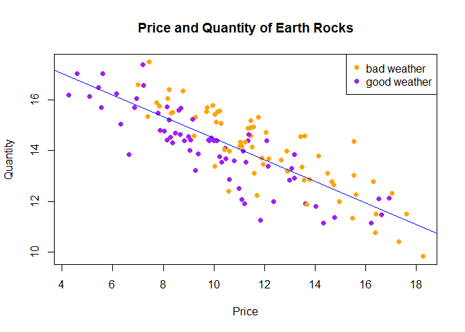
We can add the estimated demand curve from above to the plot, by using the abline() function after calling the plot() function:
plot(x = rocks$price, y = rocks$quantity,
     main = "Price and Quantity of Earth Rocks",
     xlab = "Price",
     ylab = "Quantity",
     pch = 16,
     col = rocks$mycol)

legend("topright",
       legend = c("bad weather", "good weather"),
       col=c("orange", "purple"), pch=16)

abline(lm(quantity ~ price, data = rocks), col = "blue")
