Assignment 4 Answer Key
Question 1
(a)
did <- read.csv("https://rtgodwin.com/data/card.csv")
did.mod <- lm(EMP ~ STATE + TIME + STATE * TIME + CO_OWNED, data = did)
summary(did.mod)
Coefficients:
            Estimate Std. Error t value Pr(>|t|)
(Intercept)  24.3025     1.1169  21.759  < 2e-16 ***
STATE        -2.9418     1.2141  -2.423 0.015625 *
TIME         -2.2833     1.5403  -1.482 0.138637
CO_OWNED     -2.6611     0.7141  -3.727 0.000208 ***
STATE:TIME    2.7500     1.7170   1.602 0.109659
---
Signif. codes:  0 ‘***’ 0.001 ‘**’ 0.01 ‘*’ 0.05 ‘.’ 0.1 ‘ ’ 1

Residual standard error: 9.432 on 763 degrees of freedom
Multiple R-squared:  0.02533,	Adjusted R-squared:  0.02022
F-statistic: 4.957 on 4 and 763 DF,  p-value: 0.0005991
The CO_OWNED variable helps control for differences in the treatment and control groups. The parallel trends assumption says that the treatment and control groups must be identical (except for the minimum wage policy), but this is not realistic. Additional control variables, like CO_OWNED, help establish parallel trends.
(b)
The DiD estimate is the coefficient on the interaction term: 2.75.
(c)
In general, once we start adding additional control variables like CO_OWNED, we can’t get the same estimate from the interaction term that we get using the table method. In this case however, we just happen to get 2.75 from both methods.
Question 2
Load the data:
cps <- read.csv("http://rtgodwin.com/data/cps1985.csv")
(a)
Estimate the model using the lm() function:
cps.mod <- lm(log(wage) ~ education + gender + age + experience, data = cps)
summary(cps.mod)
Coefficients:
            Estimate Std. Error t value Pr(>|t|)
(Intercept)  0.89621    0.69229   1.295    0.196
education    0.17746    0.11371   1.561    0.119
gendermale   0.25736    0.03948   6.519 1.66e-10 ***
age         -0.07961    0.11365  -0.700    0.484
experience   0.09234    0.11375   0.812    0.417
---
Signif. codes:  0 ‘***’ 0.001 ‘**’ 0.01 ‘*’ 0.05 ‘.’ 0.1 ‘ ’ 1

Residual standard error: 0.4525 on 529 degrees of freedom
Multiple R-squared:  0.2703,	Adjusted R-squared:  0.2648
F-statistic: 48.99 on 4 and 529 DF,  p-value: < 2.2e-16
(b)
The estimated effect of education on wage has a percentage change interpretation, since wage is in logs. Each additional year of education is associated with an approximate 17.8% increase in wage. However, with a p-value of 0.119 the effect is not significant.
(c)
If there is heteroskedasticity (instead of homoskedasticity), then the standard errors, t-statistics, and p-values, are all wrong.
We need to install two packages before we can estimate the “robust” standard errors (and associated t-statistics and p-values):
install.packages("lmtest")
library(lmtest)
install.packages("sandwich")
library(sandwich)
coeftest(cps.mod, vcov = vcovHC(cps.mod, "HC1"))
t test of coefficients:

             Estimate Std. Error t value  Pr(>|t|)
(Intercept)  0.896211   0.135704  6.6041 9.753e-11 ***
education    0.177461   0.011424 15.5345 < 2.2e-16 ***
gendermale   0.257361   0.039388  6.5340 1.507e-10 ***
age         -0.079611   0.011266 -7.0662 5.047e-12 ***
experience   0.092341   0.012371  7.4644 3.467e-13 ***
---
Signif. codes:  0 ‘***’ 0.001 ‘**’ 0.01 ‘*’ 0.05 ‘.’ 0.1 ‘ ’ 1
There are some very important differences from the output in part (a). Under heteroskedasticity, all of the variables are now statistically significant!
Question 1
Load the CPS data using:
cps <- read.csv("http://rtgodwin.com/data/cps1985.csv")
Part (a)
To estimate the model in R use:
summary(lm(log(wage) ~ education + gender + age + experience + gender*education, data=cps))
Coefficients:
                     Estimate Std. Error t value Pr(>|t|)
(Intercept)           0.53764    0.70887   0.758 0.448521
education             0.18311    0.11333   1.616 0.106753
gendermale            0.69499    0.20315   3.421 0.000672 ***
age                  -0.06472    0.11345  -0.570 0.568616
experience            0.07754    0.11355   0.683 0.494959
education:gendermale -0.03362    0.01531  -2.196 0.028545 *
---
Signif. codes:  0 ‘***’ 0.001 ‘**’ 0.01 ‘*’ 0.05 ‘.’ 0.1 ‘ ’ 1

Residual standard error: 0.4509 on 528 degrees of freedom
Multiple R-squared:  0.2769,	Adjusted R-squared:  0.2701
F-statistic: 40.44 on 5 and 528 DF,  p-value: < 2.2e-16
Part (b)
The estimated effect of education on wage is: 18.3% for women, and (0.18311 - 0.03362) 15.0% for men.
Part (c)
The interaction term is what allows for a diffenece in the effect of education on wages, between men and women. R has already tested the significance of this variable. With a p-value of 0.0286, the difference is statistically significant at the 5% level.
Question 3
Load the fish market data:
fish <- read.csv("https://rtgodwin.com/data/fish.csv")
Part (a)
Plot the data using something like:
plot(log(fish$avgprc), log(fish$totqty), xlab="log price", ylab="log quantity")
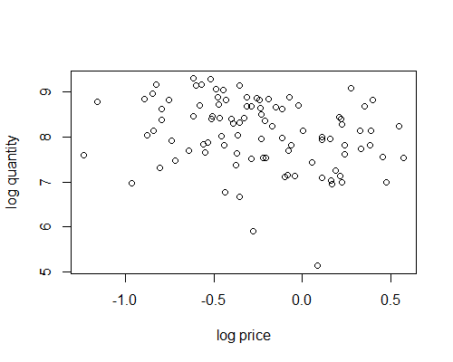
It doesn’t look like much of a demand curve. Each data point is actually the result of demand and supply intersecting, with both curves likely shifting around for each data point.
Part (b)
The population model that we are trying to estimate is:
$\log (totqty) = \beta_0 + \beta_1 \log (avgprc) + \beta_2mon + \beta_3tues + \beta_4wed + \beta_5thurs + \epsilon$
ls.fish <- lm(log(totqty) ~ log(avgprc) + mon + tues + wed + thurs, data=fish)
summary(ls.fish)
Coefficients:
            Estimate Std. Error t value Pr(>|t|)
(Intercept)  8.24432    0.16281  50.637  < 2e-16 ***
log(avgprc) -0.52466    0.17611  -2.979  0.00371 **
mon         -0.31093    0.22582  -1.377  0.17193
tues        -0.68279    0.22267  -3.066  0.00285 **
wed         -0.53389    0.21994  -2.427  0.01717 *
thurs        0.06723    0.22042   0.305  0.76107
---
Signif. codes:  0 ‘***’ 0.001 ‘**’ 0.01 ‘*’ 0.05 ‘.’ 0.1 ‘ ’ 1

Residual standard error: 0.695 on 91 degrees of freedom
Multiple R-squared:  0.2168,	Adjusted R-squared:  0.1738
F-statistic: 5.039 on 5 and 91 DF,  p-value: 0.0004025
Part (c)
We can add the estimated line to the plot using:
abline(ls.fish)
or
abline(8.24432, -0.52466)
Part (d)
The IV model that we estimated in the book (using the ivreg() function) was:
install.packages("ivreg")
library(ivreg)
iv.fish <- ivreg(log(totqty) ~ log(avgprc) + mon + tues + wed + thurs |
                             wave2 + wave3 + mon + tues + wed + thurs,
                 data = fish)
summary(iv.fish)
Coefficients:
            Estimate Std. Error t value Pr(>|t|)
(Intercept)  8.16410    0.18171  44.930  < 2e-16 ***
log(avgprc) -0.81582    0.32744  -2.492  0.01453 *
mon         -0.30744    0.22921  -1.341  0.18317
tues        -0.68473    0.22599  -3.030  0.00318 **
wed         -0.52061    0.22357  -2.329  0.02209 *
thurs        0.09476    0.22521   0.421  0.67492
We need to reproduce these results using the two-stage least-squares (2SLS) approach. In the first stage, we regress the problematic endogenous variable on the instruments and all regressors (using least-squares), and then save the LS predicted values:
stage1.mod <- lm(log(avgprc) ~ wave2 + wave3 + mon + tues + wed + thurs,
                 data=fish)
logprice.fitted <- stage1.mod$fitted.values
In the second stage, we estimate the population model using least-squares, but we replace the variable $\log (avgprc)$ with the fitted values from the first stage:
stage2.mod <- lm(log(totqty) ~ logprice.fitted + mon + tues + wed + thurs,
                 data=fish)
summary(stage2.mod)
Coefficients:
                Estimate Std. Error t value Pr(>|t|)
(Intercept)      8.16410    0.18146  44.990  < 2e-16 ***
logprice.fitted -0.81582    0.32700  -2.495  0.01440 *
mon             -0.30744    0.22890  -1.343  0.18259
tues            -0.68473    0.22569  -3.034  0.00315 **
wed             -0.52061    0.22327  -2.332  0.02192 *
thurs            0.09476    0.22490   0.421  0.67451
---
The results are nearly identical to those obtained by the ivreg() function.