R package fee

The R package fee estimates a “first-exposure effect”, its marginal effects, and standard errors. This vignette illustrates fee via an artificial data set. Please cite “Identification and estimation of a first-exposure effect in social programs” (Godwin, Simpson and Oguzoglu, 2024) when using this package.

Load package and data

The fee package requires the oneinfl package. Load both:

devtools::install_github("rtgodwin/oneinfl")
devtools::install_github("rtgodwin/fee")
library(oneinfl)
library(fee)

Load the data set:

data <- read.csv("https://rtgodwin.com/data/simdata.csv")

The data contains a continous variable $x$ and a dummy variable $d$. The data is artificial and was generated by the same process used in the simulations in Godwin, Simpson and Oguzoglu (2024).

Estimate OIZTNB and OIPP

Estimate the one-inflated zero-truncated negative binomial (OIZTNB) model:

formula <- y ~ x + d | x + d
oiztnb <- oneinfl(formula, data, dist = "negbin")
oipp <- oneinfl(formula, data, dist = "Poisson")

formula is the model to be estimated, variables that precede | link to the mean function and variables that follow | link to one-inflation. data is a data frame and dist="negbin" estimates OIZTNB while dist="Poisson" estimates OIPP. See the oneinfl package for ways in which to select between the two models.

Estimate the first-expsore effect

fee(oiztnb, data)

$where
[1] "First exposure effect averaged over all data points"

$fee
[1] -4.322372

$sefee
          [,1]
[1,] 0.2151511

$treatment_visits
[1] -4322.372

The first exposure effect has been estimated over all data points (average effects). This is the default. It is estimated that first exposure reduces the number of visits that would have occured by 4.322 (with standard error 0.215). Over a sample size of 1000, this translates to 4322 fewer ``treatment visits’’. The first exposure effect can also be estimated for the OIPP model:

fee(oipp, data)

and at the means of the data (“effect at means” or “EM”):

fee(oiztnb, data, at="EM")

Marginal effects

Estimate the marginal effects and their standard errors, for all regressors that were supplied in formula:

dfee(oiztnb, data)

$where
[1] "Marginal first exposure effect averaged over all data points"

$dfee
         x          d 
-0.5411328 -4.8098910 

$sefee
[1] 0.0601530 0.4036359

The marginal effects can also be evaluated for the OIPP model, and at the means of the variables. For example:

dfee(oipp, data, at="EM")

Plot the actual data, the factual distribution, and the counterfactual distribution

Plot the estimated factual distribution (either OIZTNB or OIPP), and the associated counterfactual distribution:

feeplot(oiztnb, data, maxpred = 12)

which produces the following plot:

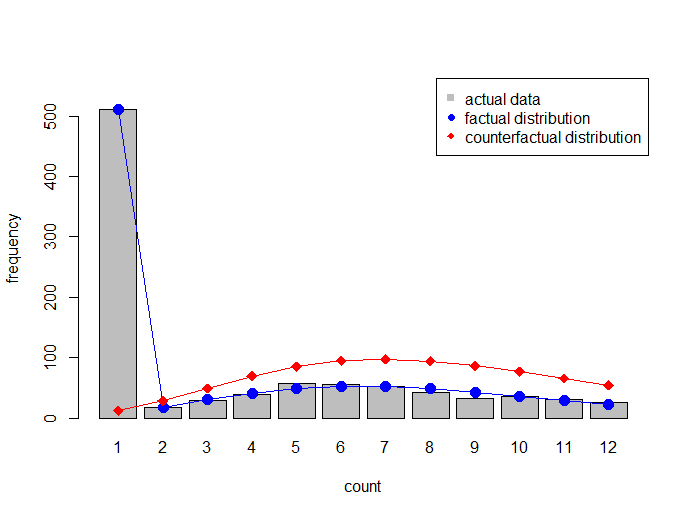
The OIPP and corresponding counterfactual distribution may be plotted using feeplot(oipp, data, maxpred = 12).

Predicted counts