Lab 1
This tutorial will start getting you accustomed to R and RStudio. Please refer to Lecture Slides 1 for information on how to install R and RStudio. R is a free software environment for statistical computing and graphics. R is one of the fastest growing programming languages in the last 5 years, and is used in a wide array of industries. R has the advantage that it is free and open-source, and that thousands of users have contributed “add-on” packages that are readily downloadable by anyone. RStudio is a free extension to R, that we will be using for the course.
Open RStudio
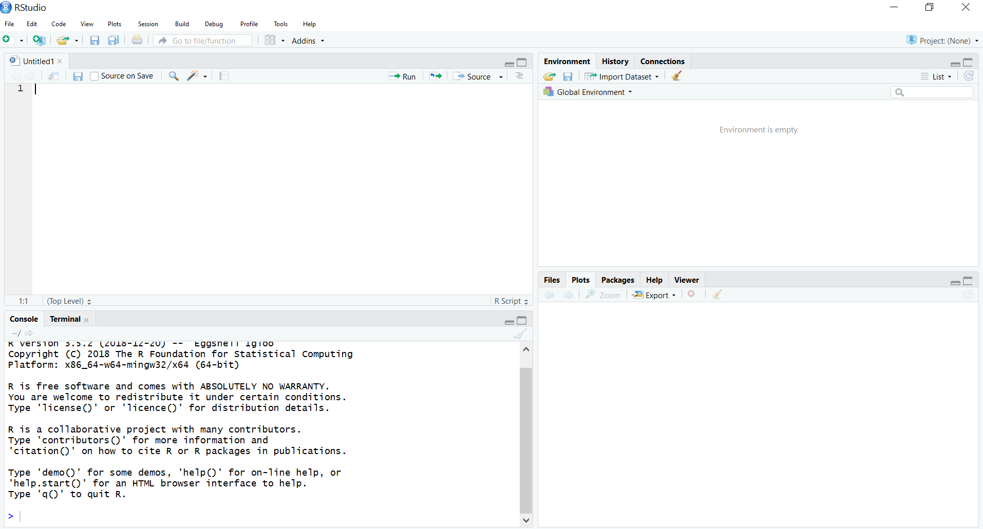
Search your computer for RStudio.exe and open the program. It should look something like this:
Create a script file
Click on “File”, “New File”, “R Script”.
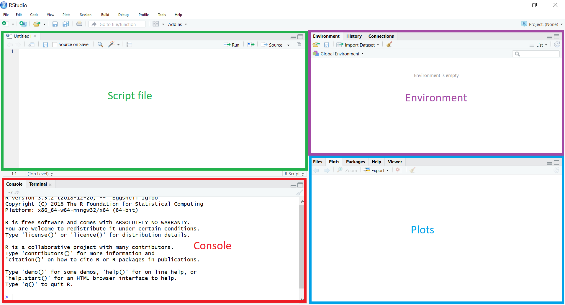
- In the top left is your Script file. R commands can be run from the R Script file, and saved at any time.
- In the bottom left is the Console window. Output is displayed here. R commands can be run from the Console, but not saved.
- In the top right is the Environment. Data and variables will be visible here.
- The bottom right will display graphics (e.g. histograms and scatterplots).
Use R as a calculator
R’s arithmetic operators include:
| Operator | Function |
|---|---|
| + | addition |
| − | subtraction |
| * | multiplication |
| / | division |
| ^ | exponentiation |
Type the following command into your R script: 1 + 2. Run the command
by highlighting it, or making sure the cursor is active at the end of
the line, and clicking ``Run’’.

Ignore the [1] that is printed out.
Create an object
You can create objects in R. Objects can be vectors, matrices, character
strings, data frames, etc. Create two different scalars (give them any
name you like, it doesn’t have to be a and b):
    a <- 3
    b <- 5
Note that you can copy-paste commands in the gray boxes directly into R.
We have created two new objects called a and b, and have assigned
them values using the assignment operator <- (the “less than” symbol
followed by the “minus” symbol). Notice that a and b pop up in the
top-right of your screen. We can now refer to these objects by name:
    a * b

    ## [1] 15
To create a vector in R we can use the “combine” function, c():
myvector <- c(1, 2, 4, 6, 7)
Simple functions in R
To call a function in R, type the name of the function, and the
arguments of the function in parentheses: functionname(arguments).
There are thousands of functions in R. Here are a few that we’ll need:
| Function |
|---|
| sum() |
| mean() |
| var() |
| summary() |
Try all of these functions on myvector. For example:
    sum(myvector)

    ## [1] 20
The sum() function is looking for arguments that it can add together.
Put an object in the brackets, and the function will try to add. Try
mean(myvector). You can get help on a function by typing ? followed
by the function name, and running the command. For example, try
?summary.
Logical operators
Logical operators are used to determine whether something is TRUE or
FALSE. Some logical operators are:
| Operator | Function |
|---|---|
| > | greater than |
| == | equal to |
| < | less than |
| >= | greater than or equal to |
| <= | less than or equal to |
| != | not equal to |
The operators & “and” and | “or” may be used to combine the above
operators.
Try entering the following commands:
    8 > 4

    ## [1] TRUE

    b == 6

    ## [1] FALSE

    b > 2

    ## [1] TRUE

    myvector > 3

    ## [1] FALSE FALSE  TRUE  TRUE  TRUE

    myvector > 3 & myvector < 7

    ## [1] FALSE FALSE  TRUE  TRUE FALSE
For the last example, R has checked to see whether each element in
myvector is greater than 3 and less than 7.
We will use these logical operators to create subsamples. We can choose certain observations in the data set based on values of the variables.
Load data
The data for this tutorial was scraped by Abdulshaheed Alqunber and is originally from (https://www.vgchartz.com/). We are using a sub sample of the data, and only look at video game sales for games making at least $100,000 USD in global sales.
The data is in the “comma-separated-format” or “.csv”. This is a very simple and common format for storing data.
RStudio can read data from your computer, or from the internet. Load the data with:
mydata <- read.csv("https://rtgodwin.com/data/vidsales.csv")
We have created a new object called mydata, and have assigned it the
values in the .csv file using the assignment operator <-. You could
have chosen a name different than mydata.
The mydata object shows up in the top-right of your screen. The sample
size is 4706 and there are 8 variables.
Click the “spreadsheet” icon next to the data set to view it. Take a
moment to look through the data, and make sure you have an idea of what
each of the variables are. The Sales variable is either the total
global sales of the game, or the sales from bundling with consoles, and
is measured in millions of US dollars. Score is the critic score from
video game reviewers, and is on a scale of 0 to 10, with 10 being best.
Notice that each video game (each observation in the data set) takes up
a different row, while the type of information on the video game (the
variables) takes up a different column. Close the “data” tab when you
are done viewing.
Explore the data
Click the blue arrow next to data in the top-right of your screen.
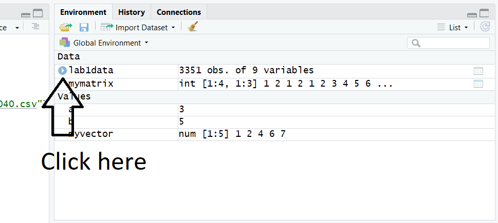
Each variable name is listed, along with some info. Notice that the variables each have a type:
| Name | Type |
|---|---|
| chr | A character string (words) |
| num | Any real (continuous) number. |
| int | Any integer. |
The “character” variables can be used to create dummy variables (more on this later!)
To explore the data, we can calculate “summary” statistics for all the variables:
    summary(mydata)

    ##      Name              Genre           ESRB_Rating          Platform
    ##  Length:4706        Length:4706        Length:4706        Length:4706
    ##  Class :character   Class :character   Class :character   Class :character
    ##  Mode  :character   Mode  :character   Mode  :character   Mode  :character
    ##
    ##
    ##
    ##   Publisher             Score           Sales             Year
    ##  Length:4706        Min.   : 1.00   Min.   : 0.010   Min.   :1985
    ##  Class :character   1st Qu.: 6.50   1st Qu.: 0.150   1st Qu.:2004
    ##  Mode  :character   Median : 7.50   Median : 0.420   Median :2008
    ##                     Mean   : 7.27   Mean   : 1.177   Mean   :2007
    ##                     3rd Qu.: 8.30   3rd Qu.: 1.100   3rd Qu.:2010
    ##                     Max.   :10.00   Max.   :82.860   Max.   :2020
The min, max, quartiles, and mean have been calculated. For example, the
sample mean Score is 7.27.
We can extract variables from the data set, and perform functions on
them. To calculate the sample variance for Sales:
    var(mydata$Sales)

    ## [1] 7.607421
Important: when we type mydata$Sales we are getting the Sales
variable from within the mydata data set.
Now, calculate the correlation between Sales and Score:
    cor(mydata$Sales, mydata$Score)

    ## [1] 0.2634555
What does this tell you?
Sub-sampling
We can use the subset() function, together with logical operators, to
create sub-samples.
Nintendo is my favourite publisher. Let’s see their critic scores vs. the critic scores from other publishers:
    mean(subset(mydata$Score, mydata$Publisher == "Nintendo"))

    ## [1] 7.799296

    mean(subset(mydata$Score, mydata$Publisher != "Nintendo"))

    ## [1] 7.21722
Notice how we have used logical operators to create two sub-samples: Nintendo games, and other games.
On your own, determine the total global sales in the data set for the publisher “Rockstar Games”.
sum(subset(mydata$Sales, mydata$Publisher == "Rockstar Games"))
Now, find all the video games that have received a perfect score of 10.
subset(mydata, mydata$Score == 10)
For the rest of the tutorial, we’ll use a sub-sample of all video games that have sales 2 million USD or more:
vid2 <- subset(mydata, mydata$Sales >= 2)
The above line creates a new data set, by selecting only the rows from
mydata which have Sales >= 2. The new data set shows up in the
top-right panel. Check the sample size.
Histograms and scatterplots
Visualization is important. Plot a histogram of critic scores:
hist(vid2$Score)
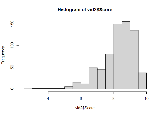
Many options are available to customize the histogram, see ?hist.
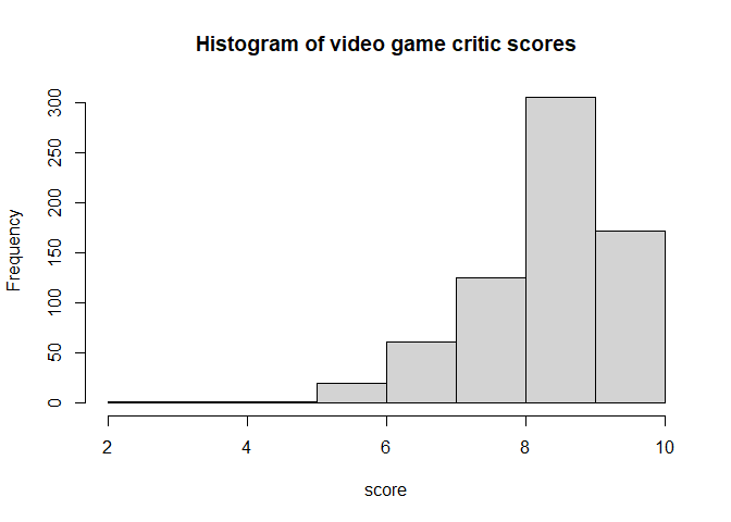
Let’s add some labels, and control the number of “breakpoints”:
    hist(vid2$Score,
         main = "Histogram of video game critic scores",
         xlab = "score",
         breaks = 10)
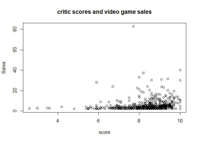
The scatterplot is a widely used tool for visualizing the relationship
between two variables. Draw a scatterplot for Sales and Score,
adding a title and labeling the axis:
    plot(vid2$Score, vid2$Sales,
         main = "critic scores and video game sales",
         xlab = "score", ylab = "Sales")
We can also change the color and style of the dots:
    plot(vid2$Score, vid2$Sales,
         col = 3,
         pch = 16)
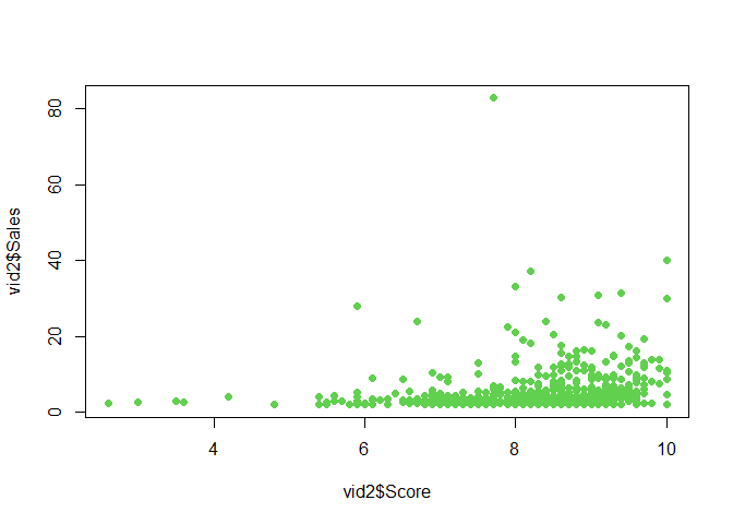
Type ?pch to see the different styles, and Google to see the different
colours.
Create new variables
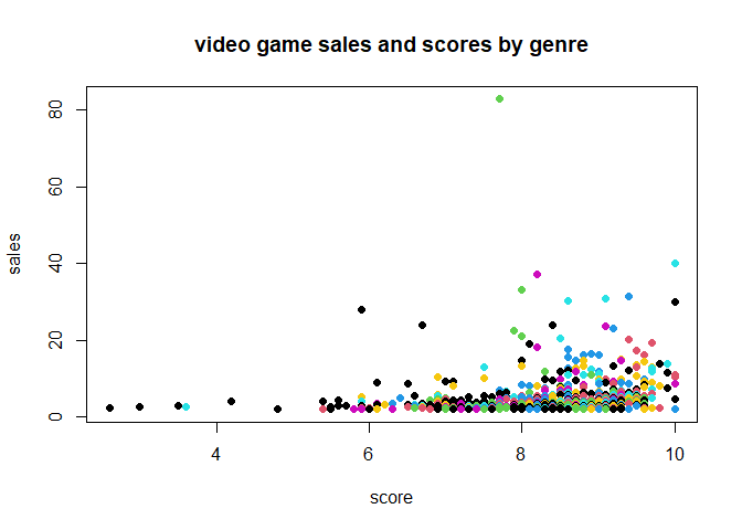
Let’s create a new variable that we’ll use to select the colour of each
data point. Make a new variable called G inside of the vid2 dataset,
and use G to control the colour of each data point. We begin by
setting all rows of the variable equal to 1, and then change the value
of G based on the game’s Genre. Copy and paste the code below:
    vid2$G <- 1
    vid2$G[vid2$Genre == "Action"] <- 2
    vid2$G[vid2$Genre == "Sports"] <- 3
    vid2$G[vid2$Genre == "Shooter"] <- 7
    vid2$G[vid2$Genre == "Role-Playing"] <- 4
    vid2$G[vid2$Genre == "Platform"] <- 5
    vid2$G[vid2$Genre == "Racing"] <- 6
For example, if Genre is equal to "Action", the variable G gets a
value of 2. Look at this G variable in the spreadsheet to understand
what has happened, Now, use this variable to determine the colour for
each data point:
    plot(vid2$Score, vid2$Sales, col=vid2$G, pch=16,
         main = "video game sales and scores by genre",
         xlab = "score", ylab = "sales")
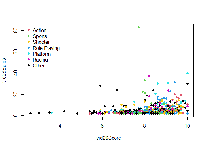
We need to add a legend to the plot to show what the colours mean:
    plot(vid2$Score, vid2$Sales, col=vid2$G, pch=16)
    legend("topleft",
           legend = c("Action", "Sports", "Shooter", "Role-Playing", "Platform", "Racing", "Other"),
           col=c(2, 3, 7, 4, 5, 6, 1), pch=16)
Import your work into Word
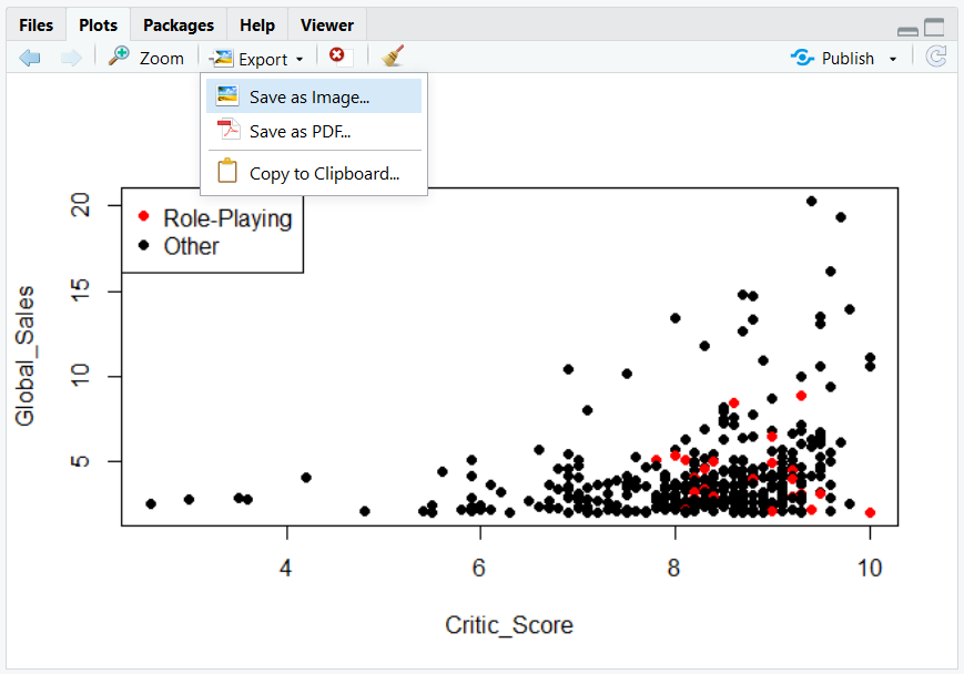
In the “plots” window, click “Export” and “Save as Image…”. This way, you can import graphics you create into Word, or another word processor.
Simple least-squares regression
What is the average increase in Sales associated with an increase in
Score? We can estimate a simple linear regression using the lm()
function (“lm” stands for “linear model”):
    lm(Sales ~ Score, data = vid2)

    ##     Call:
    ## lm(formula = Sales ~ Score, data = vid2)
    ##
    ## Coefficients:
    ## (Intercept)        Score
    ##     -2.1472       0.8912
The interpretation of the results is that an increase in critic score of 1 is associated with an average increase in sales of $0.89 million.
Save your script file
Make sure the top-left window is active, then click “File”, “Save As…”, and name your script file.
Clear your workspace
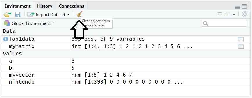
If you get too much junk floating around in R, you can clear the environment by clicking the “sweep” icon in the top-right, and start over.
